


Review Article - Journal of Contemporary Medical Education (2024)
Data Reduction Using Principal Component Analysis: Theoretical Underpinnings and Practical Applications in Public Health
Syad Hamina*Syad Hamina, Department of Medicine and Health Sciences, Hawassa University, Hawassa, Ethiopia, Email: Syadhamina@gmail.com
Received: 04-Dec-2023, Manuscript No. JCMEDU-24-124503; Editor assigned: 08-Dec-2023, Pre QC No. JCMEDU-24-124503 (PQ); Reviewed: 22-Dec-2023, QC No. JCMEDU-24-124503; Revised: 29-Dec-2023, Manuscript No. JCMEDU-24-124503 (R); Published: 05-Jan-2024
Abstract
Big datasets are becoming increasingly common and can be challenging to understand and apply in public health. One method for lowering the dimensionality of these datasets and improving interpretability while minimizing information loss is data reduction using Principal Component Analysis (PCA). It achieves this by successively maximizing variance through the creation of new, uncorrelated variables. PCA is an adaptive data analysis technique because it simplifies the process of finding new variables, or principal components, by solving an eigenvalue or eigenvector problem. These new variables are determined by the dataset being used, rather than by the analyst starting from scratch. It is also adaptable in another way because varieties of the method have been designed to adjust to various data structures and types. However, there are serious problems in the theoretical understanding and practical application of PCA among public health researchers, whereas its application is becoming more popular in developing countries. Therefore, this article, which concentrated on using PCA to reduce data, began by outlining the fundamental concepts of PCA and going over what it can and cannot do, as well as when and how to use it. This article also discussed the fundamental assumptions, benefits, and drawbacks of PCA. Furthermore, this article demonstrated and resolved PCA practical application problems in public health that most scholars are unaware of, such as variable preparation, variable inclusion and exclusion criteria for PCA, iteration steps, wealth index analysis, interpretation, and ranking.
Keywords
Principal component analysis; Data reduction; Wealth index; Public health; Eigenvalue or Eigenvector; Communality; Complex structure; Anti-image; Covariance matrix
Abbrevations
FA: Factor Analysis; ICA: Independent Component Analysis; ISOMAP: Isometric Feature Mapping; KMO: Kaiser-Meyer-Olkin; MSA: Measure of Sampling Ad- equacy; PCs: Principal Components; PCA: Principal Component Analysis; t-SNE: t-distributed Stochastic Neighbor Embedding; UAMP: Uniform Manifold Ap- proximation and Projection.
Introduction
Theoretical understanding
Data are defined as individual facts, items of information, and statistics, often numerical, that are collected using different methods [1,2]. Data, in more technical terms, is described as a set of values of quantitative and qualitative variables about one or more objects or person measurements [1,3], whereas a datum is a single value measurement assigned to a single variable [3]. Data as an overall thought refers to the fact that some prevailing knowledge or information is coded or represented in some suitable types for better processing or usage [2]. In most popular journals, data are occasionally transformed or converted into information when they are observed in context, perspective, and post-analysis [4]. But, in academic handlings of the data, they are purely units of information [5]. The data are utilized in scientific research, governance and finance (e.g., literacy, unemployment, and crime rates), business management (e.g., stock price, sales data, profits, and revenue), and almost all other types of human organizational movement (e.g., censuses of the total number of displaced people by non-profit institutions) [6-8]. Data are collected using measurement, analyzed, reported, and utilized to produce data visualizations like tables, charts, graphs, and images [9].
However, nowadays data is a heavy system, and wherever the whole thing is captured for prospect utilization, we get an enormous data set on all loads in many fields. This data set can be huge in the form of observations or interpretations and quite minuscule in the form of the number of features and columns [10,11]. The data excavating becomes tedious or mind-numbing in such cases, with merely a few significant characteristics contributing to the value that we can take out of the data [10,12]. Multifaceted or complex inquiries may take a long time and resource to go through such enormous data sets excessively [10]. In this case, a fast substitute or option is data reduction methods [10,12]. Data reduction deliberately permits us to classify or abstract the essential information from an enormous collection of data to facilitate our conscious or mindful decisions [10, 12,13].
Data reduction is the process of the transformation of alphabetical, numerical, or alphanumeric information resulting from or derived experimentally or empirically into a simplified, ordered, and corrected form [10,12-14]. In simple words, it simply means that huge volumes of data are organized, cleaned, and categorized based on predetermined criteria to support decision-making. We can utilize this idea to reduce the number of characteristics in our dataset without losing much information and to keep or improve the model’s performance. It is a powerful method to handle huge data sets without losing much information [10,12]. There are two main methods of data reduction: Dimensionality and numerosity reduction [10,12,14,15].
Literature Review
Dimensionality reduction is the procedure of decreasing the number of dimensions or sizes the data is varied across [10,12]. That means the features or attributes the data sets convey increase as the number of sizes increases. This variation is vital to outlier analysis, other algorithms, and clustering [16]. It is simple to manipulate and visualize data with reduced or decreased dimensionality [14]. Dimensionality reduction can be conducted using two different techniques. First, by merely maintaining the most significant variables from the novel dataset (this method is known as feature selection) [10]. There are six basic methods of feature selection: Missing value ratio, low variance filter, high correlation filter, random forest, backward feature elimination, and forward feature selection [10,12,14,15]. Second, by obtaining reduced sets of new variables, all being composites of the input variables and comprising fundamentally similar information with the input variables (this method is known as dimensionality reduction) [10,12]. There are two basic categories of dimensionality reduction component- or factor-based and projection-based [10]. The components, or factors-based dimensionality reduction, comprise three methods Factor Analysis (FA), Principal Component Analysis (PCA), and Independent Component Analysis (ICA). Lastly, the methods are based on projections like Isometric Feature Mapping (ISOMAP), t-distributed Stochastic Neighbor Embedding (t-SNE), and Uniform Manifold Approximation and Projection (UMAP) [10,12].
The numerosity reduction technique uses small types of data sets or representations, hence decreasing voluminous data [17]. There are two main types of numerosity reduction: Parametric and non-parametric [18]. The parametric technique assumes or considers a model into which the data set fits. Parametric data models are projected, and merely those parameters are deposited, and the remaining data set is rejected. For instance, a regression model can be utilized to attain parametric reduction if the data set fits the linear regression model. An alternative technique, the log-linear model, explores the association between two or more discrete characteristics [10,12,18]. The non-parametric reduction method doesn’t assume any type of model. It generates a more uniform reduction regardless of the size of the data set. However, it cannot attain a large volume of data reduction like the parametric method. There are 5 main types of non-parametric data reduction methods, such as histograms, sampling, data compression, data cube aggregation, and clustering [10,12,17,18]. This article focuses on providing comprehensive evidence on the theoretical underpinnings and practical applications of data reduction using PCA. This technique to reduce data is becoming the most popular, particularly in Low and Middle-Income Countries (LMICs), but is frequently misunderstood and misinterpreted by most scholars.
What is PCA?
PCA is one of the dimensionality reduction techniques that’s often utilized to reduce the dimensionality of huge data sets by converting an outsized set of variables into a reduced one that still comprises much of the information or knowledge within the large set [10,12]. It is the most extensively utilized method to deal with linear data [13]. Reducing the number of variables within data sets comes at the expense of accuracy; however, the pretend in dimensionality reduction is to trade a slight accuracy for ease [10]. Because a reduced data set is simple to visualize, explore, and make analyses of, it is much simpler and quicker for further analysis without extraneous variables to progress [12]. In short, the PCA is an important method to reduce the number of variables in a data set while maintaining as much of the information as possible [11]. It is a combination of the detected variables as a summary of these variables and handles individual measures or items as though they haven’t a unique error (assumes no error in measures) [19]. It doesn’t need the strict assumption of the primary construct, frequently utilized in physical science; accurate mathematical solutions are likely; and unity is introduced on the diagonal of the matrix. Also, it doesn’t assume constructs of hypothetical meaning but a simple mechanical linear arrangement that uses all the variance produced [20]. Obtaining or attaining a factor solution via PCA is an iterative procedure that frequently requires iterating the SPSS factor analysis process several times to attain an acceptable solution [20,21]. We start by recognizing a group of variables whose variance we consider can be characterized more parsimoniously or prudently by components or a lesser set of factors. The result of the PCA will express to us which variables can be symbolized by which components and which variables must be maintained as individual variables due to the fact that the factor solution doesn’t sufficiently symbolize their information [21].
Why is data reduction necessary using a PCA?
Some of the benefits of applying data reduction such as space needed to store the data, fewer data leading to less calculation or training time, some procedures do not execute well while we have large data sets (so decreasing these data needs to occur for the procedure to be useful), its diagnosis of multicollinearity by eliminating redundant characteristics, it supports in visualizing data because it is very challenging to visualize data in complex dimension so decreasing our space can permit us to plot or observe arrangements more visibly because we are attempting to decrease the data (we haven’t wanted as several factors as objects), because all new factors or components are the best linear arrangement of residual variance, data can be described comparatively well in several fewer factors than the original number of objects, and stop considering extra factors is a challenging decision [10,12-19,22].
When we should utilize PCA?
We can use PCA in three basic situations or times. First case: When we want to decrease the number of variables, but we are failing to detect which variable we don’t want to maintain in the data set. Second: When we want to check or detect if the variables are not dependent on one another. Third: When we are prepared to make independent features less amenable interpretation [23,24].
Some basic concepts and terms of PCA
• Eigenvalue: It displays the variance explained or described by that specific factor from out of the overall variance [25]. Any factor which contains an eigenvalue greater than or equal to 1 captures greater variance than a single detected variable. Thus, the factor that explains or captures most of the variance in these variables in the model should be utilized in other analyses, and the factor that captures the smallest amount of variance is usually rejected [26].
• Factor loading: Is the correlation coefficient (r) between latent common factors and observed variables. It describes the association of each variable to the principal factor [26]. By rule of thumb, the loading factor is considered as high if the value of the loading factor is >0.7 (i.e. the factor extracts an adequate amount of variance from that specific variable) [25].
• A complex structure: Happens while one variable has high correlations or loadings (0.40 or higher) on greater than one component. If variables have a complex structure, they must be rejected from the analysis. Variable is merely tested for complex structure if there is greater than one component in the output or solution. Variables loaded on merely one component are explained as having a simple structure [25,27].
• Communalities (h2): Are percentages of variance of each variable which can be described by the factors. It is a sum of squared factor loadings for the variables in a row from factor analysis and existing in the diagonal in common factor analysis [27].
• Bartlett’s test of sphericity: Is the extent of inter-correlation among objects and related to Cronbach’s alpha. It tests the null Hypothesis (Ho) in which the correlation matrix is an individuality matrix. The individuality matrix is a matrix that all off-diagonal components are 0 and all of the diagonal components are 1. We reject this null hypothesis if P<0.05 and it provides the smallest criteria that should be passed before a PCA should be carried out [27].
• Kaiser-Meyer-Olkin (KMO) is a Measure of Sampling Adequacy (MSA): And differs between values of 0 and 1. The value closer to one is better and the value of 0.5 is recommended as a minimum [27]. Interpretation for the KMO-MSA is: below 0.50 as unacceptable, in the 0.50’s as miserable, in the 0.60’s as mediocre, in the 0.70’s as middling, in the 0.80’s as meritorious, and in the 0.90 as marvelous [28].
Testing assumptions of PCA
CA is related to the Pearson correlation in the set of procedures; thus, it inherits the same limitations and assumptions. The basic assumptions of PCA are here below [21,22,25-27,29-33]:
• The variables involved must be dichotomously coded, either nominal or metric.
• The minimum required sample size must be more than 50 (if possible, more than 100).
• The ratio of a case to a variable in the data set must be five to one or higher.
• The correlation matrix values for the variables must comprise two or more correlations of 0.30 or higher.
• The variables with MSA<0.50 must be rejected from analysis (observe the anti-image output of SPSS).
• The total MSA must be 0.50 or greater (KMO>0.5).
• The Bartlett test of sphericity must be statistically significant, or P<0.05.
• It assumes a correlation or a linear association between features and is sensitive to the values of the features.
• It assumes no missing values and is not robust against outliers.
The checking of assumptions about principal components is vital to avoid the interpretation of distorted findings from computer software. The personal reasoning or controlling of a computer must be a hallmark feature of a scholar because a computer provides you with what you provided in the first place (garbage input, garbage output principle). Most researchers ignore this critical step of PCA and focus on output, which is a bad culture that ends up with distorted findings. Therefore, this article suggests that scholars should be critical and mindful at this stage. The first stage of a PCA is devoted to confirming that we meet these necessities. If we don’t meet these necessities, PCA is not suitable, and we reject the variables that violate assumptions after several iterations of the PCA analysis procedure.
Deriving or developing a factor model
The second stage of PCA emphasizes developing a factor model, or pattern of relations between components and variables, that fulfills the following necessities [21,22,27,29,33]:
• The derived or calculated components must explain 50% or greater of the variance in all of the variables, which means they have a communality value >0.50.
• All of the variables don’t have correlations or loadings >0.40 for more than one component, which means they don’t contain a complex structure.
• None of the components have merely one variable in them.
To fulfill these necessities, we reject problematic variables from the analysis, and the procedure of PCA will repeat.
Detecting variables to be utilized in further analysis
The detecting variables that can be utilized for further analysis are a basic concept that researchers should understand during their PCA. If, at the inference of this procedure [21,29],
• We have components that contain more than one variable correlating to or loading on them.
• We have components that describe at least 50 percent of the variance in the involved variables.
• We have components that jointly describe greater than 60 percent of the variance in the groups of variables; we may replace the component for the variable in further analysis.
• The variables that were rejected in the analysis would be involved independently in further analysis.
• Replacement of components for independent variables is carried out by utilizing merely the highest loading or correlating variable or by merging the variables loading on all components to produce a new variable.
Note
While assessing MSA, factor loadings, or commonalities, we neglect the sign of the value, and our decision is based on the magnitude or size of the value. Only the sign of the number shows the direction of the association. A correlation of 0.8 is just as strong as a correlation of -0.8. The negative sign shows a negative or an inverse association.
Steps to perform a PCA?
CA comprises five steps. Each step will be described below, providing extensive logical clarifications of what PCA is performing and making simpler mathematical ideas like covariance, standardization, eigenvalues, and eigenvectors without concentrating on how to calculate them.
Step 1: Normalization or standardization the sort of continuous preliminary variables
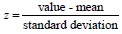
The purpose of this step is to normalize the type of continuous preliminary variables so that all of them contribute similarly to the analysis. More precisely, the rationale why it’s critical to perform normalization before PCA is that the latter is sort of sensitive concerning the variances of the preliminary variables. This means that if there is a big difference between the sorts of preliminary variables, those variables with greater variations will control over those with smaller variations (for instance, a variable that varies between 0 and 100 will control over a variable that varies between 0 and 1), which can cause biased results. Therefore, converting the variables to comparable scales can avert this problem [10,12]. Mathematically, this will be done by deducting the mean from each value and dividing by the standard deviation for every value of every variable.
Once the normalization is completed, all the variables are going to be transformed to an equivalent scale [10].
Step 2: The covariance matrix calculation
The purpose of this step is to know how the variables of the input data set are differing from the mean about one another, or, in other words, to detect if there’s any association between them [10]. Most of the time, variables are extremely correlated in such a way that they comprise redundant information [12]. Therefore, to quantify the magnitude of correlations, we calculate the covariance matrix. This covariance matrix can be a q × q symmetric matrix (q is the number of dimensions) that has all the covariance’s associated with all likely pairs of the preliminary variables. For instance, for 3-dimensional data sets with three variables such as x, y, and z, the covariance matrix can be a 3 × 3 matrix from:
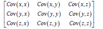
The covariance matrix for three-dimensional data meanwhile, the covariance of a data set within itself is its variance, which means Cov (x,x)=Var (x). Inside the principal diagonal, from top left to bottom right, we have the variances of each preliminary variable. Also, covariance is the property of commutativity, which means that if Cov (x,y)=Cov (y,x), then each of the covariance matrices is symmetric about the major diagonal, which suggests that the upper and therefore the lower triangular portions are identical [34]. What does the covariance that we’ve got as a total of the matrix show us regarding the relationships between the variables? It’s the sign of the covariance that determines: If it is positive, the two variables should decrease or increase together (positively correlated), and if it is negative, the one variable decreases when the opposite increases (inversely correlated) [34,35]. The covariance matrix isn’t quite a table form to summarize the associations between all the likely pairs of variables; let’s go to the subsequent step to understand more.
Step 3: Calculate the eigenvalues and eigenvectors of the covariance matrix to detect the principal components
Eigenvalues and eigenvectors are the algebraic ideas that we’d like to calculate from the covariance matrix to work out the Principal Components (PCs) of the data [36,37]. Before going to elaborate on these ideas, let’s first comprehend what we can mean by PCs. PCs are defined as new variables that are generated as linear mixtures or combinations of the preliminary variables. These mixtures are carried out such that the new variable (i.e., PCs) is not associated and most of the knowledge within the preliminary variables is compressed or squeezed into the first component. Thus, the concept is that ten-dimensional data provides you with ten PCs; however, PCA attempts to place maximum likely information within or contained by the first component, then maximum residual information within or contained by the second, and so on, up to having somewhat like presented within the figure below in the data analysis part [10,12,25-27,29]. Arranging information within PCs in this manner will permit you to decrease dimensionality without losing much information; this is attained by removing the PCs with low information and seeing the residual components as our new variables. A vital thing to comprehend here is that the PCs don’t have any actual meanin g and are less amenable for the interpretations since they’re generated as linear mixtures of the preliminary variables [26,27].
Now that we have comprehended what PCs mean, let’s return to eigenvectors and eigenvalues. The eigenvectors and eigenvalues are always presented in pairs, so that every eigenvector has an eigenvalue. Also, their number is equivalent to the dimensions of the data [36,37]. For instance, for three-dimensional data, there are three variables; thus, there are three eigenvectors with three resultant eigenvalues. The eigenvectors of the covariance matrix are accurately the directions of the axes anywhere there is the most variance or information present, also called PCs.
The eigenvalues are purely the coefficients linked to eigenvectors, which provide the amount of variance comprised in each PC [25]. By ordering your eigenvectors according to their eigenvalues, from lowest to highest, you get the PCs according to their significance. For instance, let’s assume that the data sets are two-dimensional with two variables x and y, and the eigenvectors and eigenvalues of the covariance matrix are as follows:
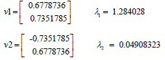
If we order the eigenvalues in decreasing order, we get λ2<λ1, which means the eigenvector that matches the PC1 is v1, and the one that matches the PC2 is v2. After obtaining the PCs, to calculate the proportion of information or variance included in each component, we simply divide the eigenvalue of each PC by the totality of eigenvalues. If we use this on the above hypothetical data, we obtain that PC2 and PC1 carry 4% and 96% of the variance of the data set, respectively.
Step 4: Generate a feature vector to choose which principal components to retain
As we discussed within the prior step, calculating the eigenvectors and ranking them by their eigenvalues in decreasing order permits us to search out the PCs of significance. The purpose of this step is to decide whether to maintain these components or reject them with less significant eigenvalues, that is, components with low eigenvalues, and produce with the residual ones a matrix of vectors that we termed a feature vector [27]. Thus, the feature vector is an unbiased matrix that has pillars, the eigenvectors of the PCs that we propose to maintain. This plan is the first step in the dimensionality reduction process. If we select to maintain only x eigenvectors or components out of y, the final data sets will have merely x dimensions [25,27]. For instance, continuing with the occurrence from the prior step, we will produce a feature vector with both of the eigenvectors v2 and v1 or reject the eigenvector v2 because it is less significant and generate a feature vector with v1 merely. Removal of the eigenvector v2 from the model will decrease dimensionality by one unit and can subsequently lead to a loss of data in the absolute data set. But as long as v2 comprises merely 4% of the variance or information, the loss is going to be thus not significant, and we will have 96% of the variance that’s comprised by v1.
Step 5: Reorganize the data within the axes of the principal component
In the prior steps, aside from standardization, we haven’t made any changes to the data set and only chosen the principal components and generated the feature vector. However, the input data sets frequently have leftovers in the form of the first axes or the forms of the preliminary variables. The purpose of this step is to utilize the feature vector generated utilizing the eigenvectors of the covariance matrix to re-familiarize the data from the original axes to those represented by the PCs, hence called the PCA. This can be carried out by multiplying the transpose of the feature vector by the transpose of the first data set [10,12].
Advantages and disadvantages of PCA
PCA has several advantages. Among these, it rejects correlated features, improves system performance, decreases or overcomes data over-fitting problems, improves data visualization, has the solvable equation that means “math is right,” is simple to calculate because it is based on linear algebra, increases the speed of other machine and model learning procedures and stabilizes the questions of big-dimensional data [23,24]. PCA provides several benefits or advantages; however, it also suffers from certain weaknesses, such as individual variables becoming less amenable for interpretation or less interpretability of PCs, data standardization or normalization being a must before doing PCA, grouping garbage data together and providing garbage outputs, making it difficult to assess the covariance in the correct method, and the issues between dimensionality reduction and information loss [23,24].
Practical application of PCA
Variable preparation for PCA: Variable preparation for PCA is the first step following data collection, and all variables can be included in PCA after careful preparation. However, many scholars have misunderstandings about the variables to be included in PCA, and most perceive that only dichotomous variables or binary variables in the form of yes/no questions assigned one and zero scores are acceptable for PCA. Due to this perception, they frequently discard collected data in the form of multiple responses, discrete numerical data, and continuous data. To avoid this misunderstanding in the following section, this article focuses on demonstrating how different types of variables will be rewritten for PCA before the main analysis. This article used a study questionnaire that contained questions about different types of variables and was designed to collect and analyze data from previous published work to facilitate the demonstration (see supporting information file 1). The multiple response variables were categorized into binary responses (yes/no) and “I don’t know” responses, often coded as 999 to zero (Table 1). Similarly, the “I don’t know” response and any missing value are often coded as 999 to zero for the continuous variables [38]. We cannot include all repapered variables in PCA that might distort our PCA results. Thus, after variable preparation, we will check the amount of variation between households using frequency descriptive analysis for all variables. Any variables or assets that were owned by households less than 5% or greater than 95% don’t clearly demonstrate an adequate amount of variation between households, and those variables should be excluded from PCA. In other words, it means the households are similar with respect to the variables owned by more than 95% or less than 5% in that particular society. The predictors that can differentiate between comparatively “poor” and “rich” households were selected using simple frequency analysis. Thus, our PCA didn’t comprise any assets or variables that were possessed by less than 5% or more than 95% of the individuals in the sample [38,39].
| S.no | Variables | Given values |
|---|---|---|
| 1 | Main source of drinking water | Improved: Piped water, tube well or borehole, protected well, protected spring=1 Unimproved: Unprotected well, Surface water (river and dam), Unprotected spring, Lake/pond/stream/canal=0 |
| 2 | Main source of water used for other purposes such as cooking and hand washing | Improved: Piped water, tube well or borehole, protected well, protected spring=1 Unimproved: Unprotected well, Unprotected spring, Lake/pond/stream/canal, Surface water (River/dam)=0 |
| 3 | Where is that water source located? | In own dwelling or yard/plot=1 Elsewhere=0 |
| 4 | Type of toilet facilities | Improved: Comprise any non-shared toilet of the subsequent kinds: Pour/flush toilets to septic tanks, piped sewer systems, and pit latrines; pit latrines with slabs; ventilated improved pit (VIP) latrines; and composting toilets=1 Unimproved: Pit latrine without slab/open pit, bucket toilet and hanging toilet=0 |
| 5 | Where is this toilet facility located? | In own dwelling or yard/plot=1 Elsewhere=0 |
| 6 | Type of fuel the household mainly use for cooking | Clean fuels include electricity, liquefied petroleum gas (LPG), natural gas, kerosene, and biogas=1 Solid fuels include coal, charcoal, wood, straw/shrub/grass, agricultural crops, and animal dung=0 |
| 7 | Where is the cooking usually done? | In the house and outdoors=0 In a separate building=1 |
| 8 | Who is the owner of the house? | Me=1 Rental, family, and relative=0 |
| 9 | Main material of the roof of the house | Natural roofing (no roof, mud, and sod)=0 Rudimentary and finished roofing=1 |
| 10 | Main material of the floor of the house | Natural floor (Earth/sand, dung)=0 Rudimentary and finished floor=1 |
| 11 | Main material of the wall of the house | Natural walls (no walls, cane/palm/trunks/bamboo, dirt)=0 Rudimentary and finished wall=1 |
| 12 | All other categorical variables were considered as yes and no form | Yes=1 and no=0 |
| 13 | All continuous variables were treated as continuous | |
| 14 | “I don’t know” response often coded as 999 for categorical variables | 999=0 |
| 15 | “I don’t know” response and any missing value often coded as 999 to zero for continuous variables | 999 and missing value=0 |
| Descriptive statistics | Mean | Std. deviation | Analysis N |
|---|---|---|---|
| have_television_in_house | .02 | .132 | 622 |
| have_radio_in_house | .37 | .484 | 622 |
| roofing_material_for_house | .67 | .472 | 622 |
| floor_material_for_house | .82 | .38 | 622 |
| wall_material_for_house | .84 | .368 | 622 |
| have_cow | .68 | .466 | 622 |
| have_ox | .46 | .499 | 622 |
| have_donkey | .05 | .221 | 622 |
| have_goat | .18 | .382 | 622 |
| have_sheep | .24 | .426 | 622 |
| have_hen | .24 | .429 | 622 |
| have_you_farm_land | .99 | .08 | 622 |
| have_bank_books_any_of_family_member | .08 | .27 | 622 |
| have_you_mobile | .37 | .483 | 622 |
| have_you_moter | .13 | .339 | 622 |
| main_sourse_of_drinking_water | .78 | .415 | 622 |
| total_duration_to_get_water | .83 | .378 | 622 |
| have_you_toilet_facility | .72 | .448 | 622 |
| how_often_family_use_toilet | .57 | .496 | 622 |
| Kaiser-Meyer-Olkin | Bartlett's test of approx | |
|---|---|---|
| Measure of sampling adequacy | .765 | |
| Chi-square sphericity | 3745.338 | |
| Df | 171 | |
| Sig. | 0 |
| Total variance explained | Initial eigenvalues | Extraction sums of squared loadings | ||||
|---|---|---|---|---|---|---|
| Component | Total | % of Variance | Cumulative % | Total | % of Variance | Cumulative % |
| 1 | 4.432 | 23.328 | 23.328 | 4.432 | 23.328 | 23.328 |
| 2 | 2.084 | 10.97 | 34.298 | 2.084 | 10.970 | 34.298 |
| 3 | 1.558 | 8.202 | 42.500 | 1.558 | 8.202 | 42.500 |
| 4 | 1.242 | 6.539 | 49.039 | 1.242 | 6.539 | 49.039 |
| 5 | 1.069 | 5.626 | 54.665 | 1.069 | 5.626 | 54.665 |
| 6 | 1.041 | 5.477 | 60.142 | 1.041 | 5.477 | 60.142 |
| 7 | .989 | 5.204 | 65.346 | |||
| 8 | .910 | 4.792 | 70.138 | |||
| 9 | .894 | 4.704 | 74.842 | |||
| 10 | .805 | 4.239 | 79.081 | |||
| 11 | .763 | 4.018 | 83.099 | |||
| 12 | .590 | 3.106 | 86.204 | |||
| 13 | .564 | 2.966 | 89.171 | |||
| 14 | .522 | 2.745 | 91.916 | |||
| 15 | .468 | 2.462 | 94.379 | |||
| 16 | .380 | 2.000 | 96.379 | |||
| 17 | .350 | 1.843 | 98.221 | |||
| 18 | .255 | 1.344 | 99.566 | |||
| 19 | .082 | .434 | 100.000 | |||
| Communalities | Initial | Extraction |
| have_television_in_house | 1.000 | .663 |
| have_radio_in_house | 1.000 | .598 |
| roofing_material_for_house | 1.000 | .468 |
| floor_material_for_house | 1.000 | .818 |
| wall_material_for_house | 1.000 | .831 |
| have_cow | 1.000 | .668 |
| have_ox | 1.000 | .685 |
| have_donkey | 1.000 | .376 |
| have_goat | 1.000 | .676 |
| have_sheep | 1.000 | .669 |
| have_hen | 1.000 | .545 |
| have_bank_books_any_of_family_member | 1.000 | .646 |
| have_you_mobile | 1.000 | .482 |
| have_you_moter | 1.000 | .531 |
| main_sourse_of_drinking_water | 1.000 | .566 |
| total_duration_to_get_water | 1.000 | .598 |
| have_you_toilet_facility | 1.000 | .598 |
| how_often_family_use_toilet | 1.000 | .777 |
| Communalities | Initial | Extraction |
| have_television_in_house | 1.000 | .714 |
| have_radio_in_house | 1.000 | .603 |
| roofing_material_for_house | 1.000 | .483 |
| floor_material_for_house | 1.000 | .821 |
| wall_material_for_house | 1.000 | .832 |
| have_cow | 1.000 | .728 |
| have_ox | 1.000 | .737 |
| have_goat | 1.000 | .694 |
| have_sheep | 1.000 | .678 |
| have_hen | 1.000 | .534 |
| have_bank_books_any_of_family_member | 1.000 | .652 |
| have_you_mobile | 1.000 | .484 |
| have_you_moter | 1.000 | .525 |
| main_sourse_of_drinking_water | 1.000 | .563 |
| total_duration_to_get_water | 1.000 | .603 |
| have_you_toilet_facility | 1.000 | .817 |
| how_often_family_use_toilet | 1.000 | .793 |
| Communalities | Initial | Extraction |
|---|---|---|
| have_television_in_house | 1.000 | .716 |
| have_radio_in_house | 1.000 | .579 |
| floor_material_for_house | 1.000 | .816 |
| wall_material_for_house | 1.000 | .832 |
| have_cow | 1.000 | .748 |
| have_ox | 1.000 | .749 |
| have_goat | 1.000 | .694 |
| have_sheep | 1.000 | .695 |
| have_hen | 1.000 | .517 |
| have_bank_books_any_of_family_member | 1.000 | .621 |
| have_you_mobile | 1.000 | .513 |
| have_you_moter | 1.000 | .569 |
| main_sourse_of_drinking_water | 1.000 | .588 |
| total_duration_to_get_water | 1.000 | .721 |
| have_you_toilet_facility | 1.000 | .835 |
| how_often_family_use_toilet | 1.000 | .812 |
| Rotated component matrixa | Component | |||||
|---|---|---|---|---|---|---|
| 1 | 2 | 3 | 4 | 5 | 6 | |
| have_television_in_house | .073 | .023 | .089 | .018 | -.022 | -.837 |
| have_radio_in_house | .575 | .253 | .346 | -.145 | .134 | -.161 |
| floor_material_for_house | -.786 | -.137 | -.032 | -.026 | -.025 | .420 |
| wall_material_for_house | -.798 | -.114 | -.064 | -.019 | .007 | .421 |
| have_cow | .126 | .092 | .805 | .198 | .167 | -.091 |
| have_ox | .219 | .058 | .821 | -.068 | .099 | -.093 |
| have_goat | -.009 | -.039 | -.042 | .805 | .193 | -.073 |
| have_sheep | .122 | .063 | .144 | .809 | -.014 | .027 |
| have_hen | -.067 | .232 | .415 | .395 | -.319 | .170 |
| have_bank_books_any_of_family_member | .769 | .028 | .029 | .012 | .062 | .153 |
| have_you_mobile | .528 | .156 | .384 | .106 | .078 | .211 |
| have_you_moter | .736 | .002 | .124 | .106 | .021 | .035 |
| main_sourse_of_drinking_water | .111 | .369 | .174 | .178 | .605 | -.109 |
| total_duration_to_get_water | .040 | .068 | .105 | .043 | .832 | .098 |
| have_you_toilet_facility | .107 | .894 | .113 | .059 | .087 | -.023 |
| how_often_family_use_toilet | .144 | .875 | .075 | -.011 | .138 | -.018 |
Note: Rotation method: Varimax with kaiser normalization; a:Rotation converged in 6 iterations.
| Rotated component matrixa | Component | ||||
|---|---|---|---|---|---|
| 1 | 2 | 3 | 4 | 5 | |
| have_television_in_house | .072 | .039 | .065 | .030 | .900 |
| have_radio_in_house | .573 | .303 | .332 | -.154 | .173 |
| floor_material_for_house | -.703 | .176 | -.059 | -.007 | -.347 |
| have_cow | .140 | .157 | .812 | .189 | .084 |
| have_ox | .233 | .101 | .820 | -.083 | .087 |
| have_goat | -.008 | .048 | -.023 | .827 | .088 |
| have_sheep | .127 | .062 | .162 | .793 | -.060 |
| have_hen | -.068 | .095 | .430 | .333 | -.281 |
| have_bank_books_any_of_family_member | .795 | .044 | -.001 | .009 | -.091 |
| have_you_mobile | .582 | .173 | .330 | .110 | -.111 |
| have_you_moter | .780 | .011 | .075 | .110 | .071 |
| main_sourse_of_drinking_water | .114 | .551 | .192 | .211 | .141 |
| have_you_toilet_facility | .094 | .889 | .100 | .033 | -.037 |
| how_often_family_use_toilet | .138 | .874 | .058 | -.033 | -.023 |
Note:Rotation method: Varimax with kaiser normalization; a:Rotation converged in 5 iterations.
Discussion
Practical demonstration of PCA using a sample data set
The sample data set was actual data collected to calculate the wealth index based on 19 variables. These 19 variables relate to ownership of carefully selected household assets like the owner of the house, television, radio, mobile, motorcycle, materials used for house construction (wall, roof, and floor), the number of rooms in a house, the presence and size of farmland, the presence of herds or farm animals and livestock (cows, oxen, donkeys, goats, and hens), and the possession and utilization of improved sanitation and water facilities.
Analysis of PCA using SPSS
After you open the sample data set for this demonstration, provide supporting information. Click on analyse

Then insert all eligible variables under the variables box. Click on descriptive, then mark on univariate descriptives, coefficients, anti-image, KMO and Bartlett’s test sphericity. Click on extraction, then method fix on principal components, mark on scree plot, and covariance matrix. Click on rotation and mark on varimax. Click on continue, and finally, click on the OK button. For further clarification, see this demonstration sample data set and my Amharic language PCA demonstration video.
First output (descriptive statistics)
Table 2 helps us check the three assumptions of PCA: First, PCA assumes the minimum sample size should be preferably greater than 100 (in this case, the sample size is 622). Second, there is no missing value for all variables (the second assumption is met). Third, the ratio of cases to variables should be 5 to 1 or greater (in this case, 31 to 1) (Table 2).
Second output (anti-image)
This table is intended to check the suitability of factor analysis or the presence of significant correlations. However, I am automatically unable to put a table in the space provided because it is too long and contains 19 variables. The PCA assumes or needs more than 2 correlations greater than or equal to 0.30 among the variables in the analysis. In this case, there are many correlations in the matrix greater than 0.30, fulfilling this assumption. The correlation matrix which is greater than 0.30 in anti-image Table is expected to be highlighted in yellow color at the time of video demonstration.
Third output (KMO and Bartlett’s Test)
This table contains two important assumptions of PCA. First, the overall Measure of Sampling Adequacy (MSA) for each variable must be >0.5 (in this case, the KMO-MSA is 0.77 and the condition is satisfied). Second, Bartlett’s Test of Sphericity must be statistically significant (here is a value less than 0.001, which indicates highly significant) (Table 3). However, on the first iteration, the MSA for the variable “owning of farmland” was 0.44, which is less than 0.5; hence, it was removed from the analysis by looking at the anti- image. On the second iteration, the MSA for each of the variables in the analysis was >0.5, which supports maintenance in the analysis. Hence, the remaining 18 variables in the analysis fulfill the criteria for the suitability of factor analysis. The subsequent step is to decide the number of factors or components that should be maintained in the factor solution.
Fourth output (determining the number of factors or components to retain in the PCA)
This is one of the important steps in PCA, and there is no statistically significant test to decide the number of factors to retain. There are four criteria, such as latent root criteria, the cumulative proportion of variance criteria, scree plots, and parallel analysis. The latent root criteria use eigenvalues greater than 1 to retain factors in PCA. The cumulative proportion of variance criteria uses the cumulative variance that explained more than 60% of variation to retain factors in PCA. The scree plot is a graphical method in which we select the factors until a break in the graph (Figure 1). In the parallel analysis, the number of components to maintain will be the number of eigenvalues (randomly generated from the investigator’s data set using PCA) that are larger than the corresponding random eigenvalues. That means comparing the randomly generated eigenvalues with the SPSS output, which is larger than the corresponding random eigenvalues. Utilizing the SPSS output from the second iteration, there are six eigenvalues greater than one, and the latent root criterion for factors shows that there are two components to be extracted for this data set. Similarly, the cumulative proportion of variance criteria should need six factors to fulfill the criterion of explaining >60% of the total variance. A six-factor solution should explain 63.26% of the overall variance. Subsequently, SPSS by default extracted the number of factors shown by all methods; the initial factor solution is based on the extraction of six components (Table 4).

Figure 1. The proportion of variance or information for each of the principal components.
Fifth output (communalities)
On the second iteration, the communalities for the variable “do you have a donkey” were 0.37, which is less than 0.50. The variable was removed, and the PCA was calculated again. In this iteration stage, there were truly 3 variables that had commonalities <0.50. The variable with the least commonality value is the candidate to select for rejection or removal first from PCA (Table 5).
On the third iteration, the communality for the variable “roofing materials for the house” was 0.48, which is less than 0.5. The variable was rejected, and the PCA was calculated again (Table 6).
After all variables with communalities greater than 0.50 have been included in the analysis, the arrangement of factor loadings must be examined to detect variables that have a complex structure (Table 7). A complex structure occurs when one variable has high correlations or loadings (0.40 or higher) on more than one component. If variables have a complex structure, they must be rejected from the analysis. A variable is merely tested for complex structure if there is more than one component in the output or solution. Variables that are loaded on merely one component are explained as having a simple structure.
Sixth output (complex structure)
On the fourth iteration, the variable “the total duration to get water” contains a complex structure. In this iteration stage, there are truly 3 variables that have a complex structure>0.4. The variable with the highest complex structure value is the candidate to select for rejection or removal first. Specifically, the variable had a loading of 0.83 on component 5, and a loading of 0.40 on component 1 was rejected from the analysis. The variable should be removed, and the principal component analysis should be reiterated (Table 8).
On the 6th iteration, all of the variables haven’t revealed a complex structure. Further removal of any variables from the analysis is not required due to the complex structure. The communality for each of the variables involved in the factors was >0.50, and all variables have a simple structure (Table 9). We declare that the PCA has been finalized. The information in 14 variables can be represented or explained by 5 components. At these stages, we are confident in using the principal component to conduct the computation of the wealth index [38, 40] because the basic assumptions of PCA were checked before ranking the components’ factor scores into wealth quintiles. We removed the variables from PCA that didn’t satisfy the assumptions, such as the Kaiser-Meyer-Olkin (KMO) measure of sampling adequacy less than 0.5, commonalities less than 0.5, and variables that contain complex structures (high loading correlation >0.4 on more than one component) [40,41]. Finally, the component factors or wealth index scores were ranked into 5 classes, such as lowest, second-lowest, middle, second-highest, and highest [40,42].
Conclusion
The term data is defined as a set of values of quantitative and qualitative variables about one or more objects or persons. However, big datasets are progressively becoming a common phenomenon in several disciplines and are frequently challenging to interpret. Data reduction methods are one of the solutions to overcome such challenges. There are two major techniques of data reduction, such as dimensionality and numerosity reduction. There are two basic categories of dimensionality reduction: Component- or factor-based and projection-based.
The component, or factors-based dimensionality reduction, comprises three methods: Factor Analysis (FA), Principal Component Analysis (PCA), and Independent Component Analysis (ICA). PCA is one of the methods for decreasing the dimensionality of such large datasets and improving interpretability, while at the same time reducing information loss. Thus, it operates by producing new non-correlated variables that sequentially maximize variance. Obtaining such principal components (new variables) decreases to solving an eigenvector or eigenvalue problem, as the new variables or components are described by the data at hand, not an earlier one, thus making PCA an adaptive data analysis method. This article focused on data reduction using PCA and started by introducing the fundamental concepts of PCA, discussing what it can and cannot perform, when to use it, and how to use it. Also, we discussed the basic assumptions, advantages, and disadvantages of PCA. Furthermore, this article demonstrated and fixed the PCA practical application problems most scholars are not aware of in public health, such as variable preparation, variable inclusion and exclusion criteria for PCA, iteration steps, analysis, interpretation, and ranking of wealth index.
Therefore, this comprehensive information will help researchers easily understand the theoretical concepts and practical application in public health, particularly in LMICs where PCA is becoming popular.
Declarations
Ethics approval and consent to participate
Not applicable
Consent for publication
Not applicable
Availability of data and materials
All data generated or analyzed during this study are included in this published article and its supplementary information files.
Competing interests
Not applicable
Funding
Not applicable
Authors’ contributions
AY: Conceptualized, ensured data curation, did the formal analysis, and wrote the manuscript.
Acknowledgments
My greatest thanks go to Netsanet Kibru for her big support during the preparatieon of this article by giving her ideas.
References
- OECD P. OECD glossary of statistical terms.
- Makady A, de Boer A, Hillege H, Klungel O, Goettsch W. What is real-world data? A review of definitions based on literature and stakeholder interviews. Value Health 2017;20(7):858-865.
[Crossref] [Google Scholar] [Pubmed]
- Statistical Language-What is Data. Australian Bureau of Statistics. 2013
- Data vs Information-Difference and Comparison/Diffen. 201-12-11.
- Iris Garner. Data in education.
- Joubert J, Rao C, Bradshaw D, Dorrington RE, Vos T, Lopez A, et al. Characteristics, availability and uses of vital registration and other mortality data sources in post-democracy South Africa. Glob Health Action 2012;5(1):19263.
[Crossref] [Google Scholar] [Pubmed]
- Wyatt D, Cook J, Mckevitt C. Perceptions of the uses of routine general practice data beyond individual care in England: A qualitative study. BMJ Open 2018;8(1).
[Crossref] [Google Scholar] [Pubmed]
- Peloquin D, DiMaio M, Bierer B, Barnes M. Disruptive and avoidable: GDPR challenges to secondary research uses of data. Eur J Hum Genet 2020;28(6):697-705.
[Crossref] [Google Scholar] [Pubmed]
- Degu G, Tessema F. For health science students. 2005.
- Jyotsna Vadakkanmarveettil. Data reduction: A simple and concise guide. 2021
- Jolliffe IT, Cadima J. Principal component analysis: A review and recent developments. Philos Trans A Math Phys Eng Sci 2016;374(2065):20150202.
[Crossref] [Google Scholar] [Pubmed]
- PulkitS. The ultimate guide to 12 dimensionality reduction techniques (with python codes).2023.
- Gleason PM, Boushey CJ, Harris JE, Zoellner J. Publishing nutrition research: A review of multivariate techniques-part 3: Bata reduction methods. J Acad Nutr Diet 2015;115(7):1072-1082.
[Crossref] [Google Scholar] [Pubmed]
- Santana AC, Barbosa AV, Yehia HC, Laboissière R. A dimension reduction technique applied to regression on high dimension, low sample size neurophysiological data sets. BMC Neurosci 2021;22(1):1-4.
[Crossref] [Google Scholar] [Pubmed]
- Neha T. Data reduction.
- Rukshan Pramoditha. 11 dimensionality reduction techniques you should know in 2021.2021
- Shreysingh T. Difference between dimensionality reduction and numerosity reduction.
- Numerosity reduction in data mining. GeeksforGeeks.
- Lever J, Krzywinski M, Altman N. Points of significance: Principal component analysis. Nat Methods 2017;14(7):641-643.
- Casal CA, Losada JL, Barreira D, Maneiro R. Multivariate exploratory comparative analysis of LaLiga Teams: Principal component analysis. Int J Environ Res Public Health 2021;18(6):3176.
[Crossref] [Google Scholar] [Pubmed]
- Factor analysis. Jkljkllmn.
- Shaily Jain. Limitations, assumptions watch-outs of principal component analysis. 2021.
- Matt Brems. A one-stop shop for principal component analysis. 2017.
- Rohit Dwivedi. Introduction to principal component analysis in machine learning. 2021.
- Factor analysis. Statistics Solutions.
- Factor Analysis: A Short Introduction, Part 1. The Analysis Factor.
- Factor analysis/SPSS annotated output.
- Satish GJ, Nagesha N. A case study of barriers and drivers for energy efficiency in an Indian city. Int J Energy Technol Policy 2017;13(3):266-277.
- Principal Component Analysis. Data analysis and computers II.
- Song Y, Westerhuis JA, Aben N, Michaut M, Wessels LF, Smilde AK,et al. Principal component analysis of binary genomics data. Brief Bioinform 2019;20(1):317-329.
[Crossref] [Google Scholar] [Pubmed]
- Wang B, Luo X, Zhao Y, Caffo B. Semiparametric partial common principal component analysis for covariance matrices. Biometrics 2021;77(4):1175-1186.
[Crossref] [Google Scholar] [Pubmed]
- Santos RD, Gorgulho BM, Castro MA, Fisberg RM, Marchioni DM, Baltar VT, et al. Principal component analysis and factor analysis: Differences and similarities in nutritional epidemiology application. Rev Bras Epidemiol 2019;22: e190041.
[Crossref] [Google Scholar] [Pubmed]
- Principal Components Analysis (PCA) using SPSS statistics. Laerd Statistics.
- Nikolai Janakiev. Understanding the covariance matrix. 2018
- Stat Trek. Variance-covariance matrix.
- Hoffman K, Kunze R. Characteristic values. Linear Algebra. 1971:182-190.
- Marcus M, Minc H. Introduction to linear algebra. 1988.
- Fry KFR, Chakraborty N.M. Measuring equity with nationally representative wealth quintiles. Washington, DC: PSI. 2014.
- Ahmed R, Sultan M, Abose S, Assefa B, Nuramo A, Alemu A, et al. Levels and associated factors of the maternal healthcare continuum in Hadiya zone, Southern Ethiopia: A multilevel analysis. PLoS One 2022;17(10):e0275752.
[Crossref] [Google Scholar] [Pubmed]
- Vyas S, Kumaranayake L. Constructing socio-economic status indices: How to use principal components analysis. Health Policy Plan 2006;21(6):459-468.
[Crossref] [Google Scholar] [Pubmed]
- Principal component analysis.
- Central Statistical Agency (CSA) (Ethiopia) and ICF. Mini Ethiopia Demographic and Health Survey 2019: Key Indicators Report. 2019.